How To Assess Linear Regression
March 27, 2019
衡量回归算法的标准
将测试数据集带入计算损失函数
\[\sum_{i=0}^m(y_{test}^{(i)} - \hat{y}_{test}^{(i)})^2\]问题:结果和 m 有关
均方误差MSE
\(\frac{1}{m}\sum_{i=0}^m(y_{test}^{(i)} - \hat{y}_{test}^{(i)})^2\) 问题:结果受量纲影响
均方根误差RMSE
\[\sqrt{\frac{1}{m}\sum_{i=0}^m(y_{test}^{(i)} - \hat{y}_{test}^{(i)})^2} = \sqrt{MSE_{test}}\]平均绝对误差MAE
\[\frac{1}{m}\sum_{i=0}^m|y_{test}^{(i)} - \hat{y}_{test}^{(i)}|\]波士顿房产数据
import numpy as np
import matplotlib.pyplot as plt
from sklearn import datasets

boston = datasets.load_boston()
print(boston.DESCR)
Boston House Prices dataset
===========================

Notes
------
Data Set Characteristics:

    :Number of Instances: 506

    :Number of Attributes: 13 numeric/categorical predictive

    :Median Value (attribute 14) is usually the target

    :Attribute Information (in order):
        - CRIM     per capita crime rate by town
        - ZN       proportion of residential land zoned for lots over 25,000 sq.ft.
        - INDUS    proportion of non-retail business acres per town
        - CHAS     Charles River dummy variable (= 1 if tract bounds river; 0 otherwise)
        - NOX      nitric oxides concentration (parts per 10 million)
        - RM       average number of rooms per dwelling
        - AGE      proportion of owner-occupied units built prior to 1940
        - DIS      weighted distances to five Boston employment centres
        - RAD      index of accessibility to radial highways
        - TAX      full-value property-tax rate per $10,000
        - PTRATIO  pupil-teacher ratio by town
        - B        1000(Bk - 0.63)^2 where Bk is the proportion of blacks by town
        - LSTAT    % lower status of the population
        - MEDV     Median value of owner-occupied homes in $1000's

    :Missing Attribute Values: None

    :Creator: Harrison, D. and Rubinfeld, D.L.

This is a copy of UCI ML housing dataset.
http://archive.ics.uci.edu/ml/datasets/Housing


This dataset was taken from the StatLib library which is maintained at Carnegie Mellon University.

The Boston house-price data of Harrison, D. and Rubinfeld, D.L. 'Hedonic
prices and the demand for clean air', J. Environ. Economics & Management,
vol.5, 81-102, 1978.   Used in Belsley, Kuh & Welsch, 'Regression diagnostics
...', Wiley, 1980.   N.B. Various transformations are used in the table on
pages 244-261 of the latter.

The Boston house-price data has been used in many machine learning papers that address regression
problems.

**References**

   - Belsley, Kuh & Welsch, 'Regression diagnostics: Identifying Influential Data and Sources of Collinearity', Wiley, 1980. 244-261.
   - Quinlan,R. (1993). Combining Instance-Based and Model-Based Learning. In Proceedings on the Tenth International Conference of Machine Learning, 236-243, University of Massachusetts, Amherst. Morgan Kaufmann.
   - many more! (see http://archive.ics.uci.edu/ml/datasets/Housing)
boston.feature_names
array([‘CRIM’, ‘ZN’, ‘INDUS’, ‘CHAS’, ‘NOX’, ‘RM’, ‘AGE’, ‘DIS’, ‘RAD’, ‘TAX’, ‘PTRATIO’, ‘B’, ‘LSTAT’], dtype=’<U7’)
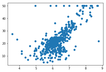
x = boston.data[:,5] # 暂时只使用房间的数量
y = boston.target
plt.scatter(x, y)
plt.show()
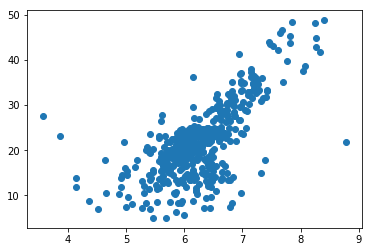
np.max(y)
50.0
x = x[y < 50]
y = y[y < 50]
plt.scatter(x, y)
plt.show()
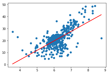
x_train, x_test, y_train, y_test = train_test_split(x, y, seed=666)
slr = SimpleLinearRegressionV2()
slr.fit(x_train, y_train)
SimpleLinearRegressionV2()
plt.scatter(x_train, y_train)
plt.plot(x_train, slr.predict(x_train), color='r')
[<matplotlib.lines.Line2D at 0x937cb00>]
y_predict = slr.predict(x_test)
MSE
mse_test = np.sum((y_test - y_predict) ** 2) / len(x_test)
mse_test
24.156602134387438
RMSE
rmse_test = np.sqrt(mse_test)
rmse_test
4.914936635846635
MAE
mae_test = np.sum(np.abs(y_test - y_predict)) / len(x_test)
mae_test
3.5430974409463873
使用自己封装的函数
def mean_squared_error(y_true, y_predict):
    assert len(y_true) == len(y_predict),\
        "the size of y_true must be equal to the size of y_predict"
    return np.sum((y_true - y_predict) ** 2) / len(y_true)

def root_mean_squared_error(y_true, y_oredict):
    return np.sqrt(mean_squared_error(y_true, y_oredict))

def mean_absolute_error(y_true, y_predict):
    assert len(y_true) == len(y_predict),\
        "the size of y_true must be equal to the size of y_predict"
    return np.sum(np.abs(y_true - y_predict)) / len(y_true)
mean_squared_error(y_test, y_predict)
24.156602134387438
root_mean_squared_error(y_test, y_predict)
4.914936635846635
mean_absolute_error(y_test, y_predict)
3.5430974409463873
scikit-lean 中的 MSE 和MAE
from sklearn.metrics import mean_squared_error, mean_absolute_error
mean_squared_error(y_test, y_predict)
24.156602134387438
np.sqrt(mean_squared_error(y_test, y_predict))
4.914936635846635
mean_absolute_error(y_test, y_predict)
3.5430974409463873
R Square
见下节