Logistic Regression Implement And Decision Boundary
April 30, 2019
实现逻辑回归
import numpy as np
import matplotlib.pyplot as plt
from sklearn import datasets
iris = datasets.load_iris()

X = iris.data
y = iris.target
X = X[y<2,:2]
y = y[y<2]
X.shape
(100, 2)
y.shape
(100,)
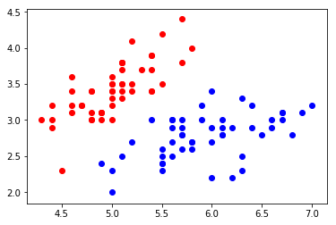
plt.scatter(X[y==0,0], X[y==0,1], color="red")
plt.scatter(X[y==1,0], X[y==1,1], color="blue")
plt.show()
使用逻辑回归
LogisticRegression.py
import numpy as np

def accuracy_score(y_true, y_predict):
    assert y_true.shape == y_predict.shape,\
        "the size of y_true must be equal to the size of y_predict"
    return (sum(y_true == y_predict) / len(y_true))

class LogisticRegression:

    def __init__(self):
        """初始化Logistic Regression模型"""
        self.coef_ = None
        self.intercept_ = None
        self._theta = None

    def _sigmoid(self, t):
        return 1. / (1. + np.exp(-t))

    def fit(self, X_train, y_train, eta=0.01, n_iters=1e4):
        """根据训练数据集X_train, y_train, 使用梯度下降法训练Logistic Regression模型"""
        assert X_train.shape[0] == y_train.shape[0], \
            "the size of X_train must be equal to the size of y_train"

        def J(theta, X_b, y):
            y_hat = self._sigmoid(X_b.dot(theta))
            try:
                return - np.sum(y*np.log(y_hat) + (1-y)*np.log(1-y_hat)) / len(y)
            except:
                return float('inf')

        def dJ(theta, X_b, y):
            return X_b.T.dot(self._sigmoid(X_b.dot(theta)) - y) / len(y)

        def gradient_descent(X_b, y, initial_theta, eta, n_iters=1e4, epsilon=1e-8):

            theta = initial_theta
            cur_iter = 0

            while cur_iter < n_iters:
                gradient = dJ(theta, X_b, y)
                last_theta = theta
                theta = theta - eta * gradient
                if (abs(J(theta, X_b, y) - J(last_theta, X_b, y)) < epsilon):
                    break

                cur_iter += 1

            return theta

        X_b = np.hstack([np.ones((len(X_train), 1)), X_train])
        initial_theta = np.zeros(X_b.shape[1])
        self._theta = gradient_descent(X_b, y_train, initial_theta, eta, n_iters)

        self.intercept_ = self._theta[0]
        self.coef_ = self._theta[1:]

        return self

    def predict_proba(self, X_predict):
        """给定待预测数据集X_predict,返回表示X_predict的结果概率向量"""
        assert self.intercept_ is not None and self.coef_ is not None, \
            "must fit before predict!"
        assert X_predict.shape[1] == len(self.coef_), \
            "the feature number of X_predict must be equal to X_train"

        X_b = np.hstack([np.ones((len(X_predict), 1)), X_predict])
        return self._sigmoid(X_b.dot(self._theta))

    def predict(self, X_predict):
        """给定待预测数据集X_predict,返回表示X_predict的结果向量"""
        assert self.intercept_ is not None and self.coef_ is not None, \
            "must fit before predict!"
        assert X_predict.shape[1] == len(self.coef_), \
            "the feature number of X_predict must be equal to X_train"

        proba = self.predict_proba(X_predict)
        return np.array(proba >= 0.5, dtype='int')

    def score(self, X_test, y_test):
        """根据测试数据集 X_test 和 y_test 确定当前模型的准确度"""

        y_predict = self.predict(X_test)
        return accuracy_score(y_test, y_predict)

    def __repr__(self):
        return "LogisticRegression()"
from sklearn.model_selection import train_test_split
X_train, X_test, y_train, y_test = train_test_split(X, y, seed=666)
log_reg = LogisticRegression()
log_reg.fit(X_train, y_train)
LogisticRegression()
log_reg.score(X_test, y_test)
1.0
log_reg.predict_proba(X_test)
array([0.92972035, 0.98664939, 0.14852024, 0.17601199, 0.0369836 , 0.0186637 , 0.04936918, 0.99669244, 0.97993941, 0.74524655, 0.04473194, 0.00339285, 0.26131273, 0.0369836 , 0.84192923, 0.79892262, 0.82890209, 0.32358166, 0.06535323, 0.20735334])
y_test
array([1, 1, 0, 0, 0, 0, 0, 1, 1, 1, 0, 0, 0, 0, 1, 1, 1, 0, 0, 0])
log_reg.predict(X_test)
array([1, 1, 0, 0, 0, 0, 0, 1, 1, 1, 0, 0, 0, 0, 1, 1, 1, 0, 0, 0])
log_reg.coef_
array([ 3.01796521, -5.04447145])
log_reg.intercept_
-0.6937719272911228
决策边界
\[\hat{p }= \sigma(\theta^T \cdot x_b) = \frac{1}{1 + e^{-\theta^T \cdot x_b}}\] \[\hat{y} = \begin{cases} 1,\quad \hat{p} \geq 0.5 \quad \theta^T \cdot x_b \geq 0\\\\ 0,\quad \hat{p} < 0.5 \quad \theta^T \cdot x_b < 0 \end{cases}\]此时$\theta^T \cdot x_b = 0$为决策边界
如果X有两个特征,可以写作$\theta_0 + \theta_1x_1 + \theta_2x_2 = 0$
或者写作
\[x_2 = \frac{-\theta_0 - \theta_1x_1}{\theta_2}\]可以表达为一条实线
def x2(x1):
    return (-log_reg.coef_[0] * x1 - log_reg.intercept_) / log_reg.coef_[1]
x1_plot = np.linspace(4, 8, 1000)
x2_plot = x2(x1_plot)
plt.scatter(X[y==0,0], X[y==0,1], color="red")
plt.scatter(X[y==1,0], X[y==1,1], color="blue")
plt.plot(x1_plot, x2_plot)
plt.show()
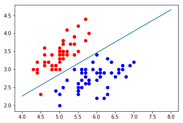
这根线就是我们说的决策边界
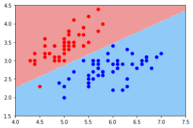
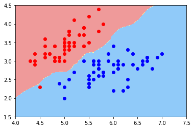
绘制不规则的决策边界
from matplotlib.colors import ListedColormap

def plot_decision_boundary(model, axis):
    x0, x1 = np.meshgrid(
        np.linspace(axis[0], axis[1], int((axis[1] - axis[0]) * 100 )).reshape(-1, 1),
        np.linspace(axis[2], axis[3], int((axis[3] - axis[2]) * 100 )).reshape(-1, 1)
    )
    X_new = np.c_[x0.ravel(), x1.ravel()]

    y_predict = model.predict(X_new)
    zz = y_predict.reshape(x0.shape)

    custom_camp = ListedColormap(['#EF9A9A', '#FFF59F', '#90CAF9'])
    plt.contourf(x0, x1, zz, cmap=custom_camp)
plot_decision_boundary(log_reg, axis=[4, 7.5, 1.5, 4.5])
plt.scatter(X[y==0,0], X[y==0,1], color="red")
plt.scatter(X[y==1,0], X[y==1,1], color="blue")
plt.show()
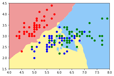
kNN 的决策边界
from sklearn.neighbors import KNeighborsClassifier

knn_clf = KNeighborsClassifier()
knn_clf.fit(X_train, y_train)
KNeighborsClassifier(algorithm=’auto’, leaf_size=30, metric=’minkowski’, metric_params=None, n_jobs=1, n_neighbors=5, p=2, weights=’uniform’)
knn_clf.score(X_test, y_test)
1.0
plot_decision_boundary(knn_clf, axis=[4, 7.5, 1.5, 4.5])
plt.scatter(X[y==0,0], X[y==0,1], color="red")
plt.scatter(X[y==1,0], X[y==1,1], color="blue")
plt.show()
knn_clf_all = KNeighborsClassifier()
knn_clf_all.fit(iris.data[:,:2], iris.target)
KNeighborsClassifier(algorithm=’auto’, leaf_size=30, metric=’minkowski’, metric_params=None, n_jobs=1, n_neighbors=5, p=2, weights=’uniform’)
plot_decision_boundary(knn_clf_all, axis=[4, 8, 1.5, 4.5])
plt.scatter(iris.data[iris.target==0,0], iris.data[iris.target==0,1], color="red")
plt.scatter(iris.data[iris.target==1,0], iris.data[iris.target==1,1], color="blue")
plt.scatter(iris.data[iris.target==2,0], iris.data[iris.target==2,1], color="green")
plt.show()
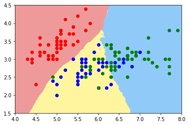
knn_clf_all = KNeighborsClassifier(n_neighbors=50)
knn_clf_all.fit(iris.data[:,:2], iris.target)
KNeighborsClassifier(algorithm=’auto’, leaf_size=30, metric=’minkowski’, metric_params=None, n_jobs=1, n_neighbors=50, p=2, weights=’uniform’)
plot_decision_boundary(knn_clf_all, axis=[4, 8, 1.5, 4.5])
plt.scatter(iris.data[iris.target==0,0], iris.data[iris.target==0,1], color="red")
plt.scatter(iris.data[iris.target==1,0], iris.data[iris.target==1,1], color="blue")
plt.scatter(iris.data[iris.target==2,0], iris.data[iris.target==2,1], color="green")
plt.show()