scikit-learn 中的多项式回归和Pipeline

import numpy as np
import matplotlib.pyplot as plt

x = np.random.uniform(-3, 3, size=100)
X = x.reshape(-1, 1)
y = 0.5 * x ** 2 + x + 2 + np.random.normal(0, 1, 100)

from sklearn.preprocessing import PolynomialFeatures

poly = PolynomialFeatures(degree=2)
poly.fit(X)
X2 = poly.transform(X)
X2.shape

(100, 3)

X2[:5]

array([[ 1. , -2.42731039, 5.89183574], [ 1. , -1.1892334 , 1.41427607], [ 1. , 2.97919223, 8.87558632], [ 1. , -0.3104026 , 0.09634978], [ 1. , -2.28611994, 5.22634437]])

X[:5]

array([[-2.42731039], [-1.1892334 ], [ 2.97919223], [-0.3104026 ], [-2.28611994]])

from sklearn.linear_model import LinearRegression

lin_reg = LinearRegression()
lin_reg.fit(X2, y)
y_predict = lin_reg.predict(X2)

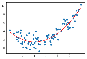
plt.scatter(x, y)
plt.plot(np.sort(x), y_predict[np.argsort(x)], color='r')
plt.show()

lin_reg.coef_

array([0. , 1.01522347, 0.48684016])

lin_reg.intercept_

1.9568056125014162

关于 PolynomialFeatures

当 degree = 3

如果原特征为

则零次项：

一次项：

二次项：

三次项：

共十项，可以看出随着 degree ，多项式项数指数级增加，功能强大，但会带来一些问题

X = np.arange(1, 11).reshape(-1, 2)

X

array([[ 1, 2], [ 3, 4], [ 5, 6], [ 7, 8], [ 9, 10]])

poly = PolynomialFeatures(degree=3)
poly.fit(X)
X3 = poly.transform(X)
X3

array([[ 1., 1., 2., 1., 2., 4., 1., 2., 4., 8.], [ 1., 3., 4., 9., 12., 16., 27., 36., 48., 64.], [ 1., 5., 6., 25., 30., 36., 125., 150., 180., 216.], [ 1., 7., 8., 49., 56., 64., 343., 392., 448., 512.], [ 1., 9., 10., 81., 90., 100., 729., 810., 900., 1000.]])

Pipeline

将多项式特征、数据归一化、线性回归三步合成一步

x = np.random.uniform(-3, 3, size=100)
X = x.reshape(-1, 1)
y = 0.5 * x ** 2 + x + 2 + np.random.normal(0, 1, 100)

from sklearn.pipeline import Pipeline
from sklearn.preprocessing import StandardScaler

poly_reg = Pipeline([
    ("poly", PolynomialFeatures(degree=2)),
    ("std_scaler", StandardScaler()),
    ("lin_reg", LinearRegression())
])

poly_reg.fit(X, y)
y_predict = poly_reg.predict(X)

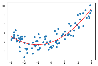
plt.scatter(x, y)
plt.plot(np.sort(x), y_predict[np.argsort(x)], color='r')
plt.show()