Practice of Svm
May 27, 2019
实际使用SVM
- 和kNN一样,要做数据标准化处理!
- 涉及距离!
import numpy as np
import matplotlib.pyplot as plt
from sklearn import datasets
iris = datasets.load_iris()
X = iris.data
y = iris.target
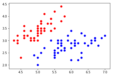
X = X[y < 2, :2]
y = y[y < 2]
plt.scatter(X[y==0,0], X[y==0,1], color='red')
plt.scatter(X[y==1,0], X[y==1,1], color='blue')
plt.show()
from sklearn.preprocessing import StandardScaler

std_scaler = StandardScaler()
std_scaler.fit(X)
X_standard = std_scaler.transform(X)
from sklearn.svm import LinearSVC

svc = LinearSVC(C=1e9)
svc.fit(X_standard, y)
LinearSVC(C=1000000000.0, class_weight=None, dual=True, fit_intercept=True, intercept_scaling=1, loss=’squared_hinge’, max_iter=1000, multi_class=’ovr’, penalty=’l2’, random_state=None, tol=0.0001, verbose=0)
from matplotlib.colors import ListedColormap

def plot_decision_boundary(model, axis):
    x0, x1 = np.meshgrid(
        np.linspace(axis[0], axis[1], int((axis[1] - axis[0]) * 100 )).reshape(-1, 1),
        np.linspace(axis[2], axis[3], int((axis[3] - axis[2]) * 100 )).reshape(-1, 1)
    )
    X_new = np.c_[x0.ravel(), x1.ravel()]

    y_predict = model.predict(X_new)
    zz = y_predict.reshape(x0.shape)

    custom_camp = ListedColormap(['#EF9A9A', '#FFF59F', '#90CAF9'])
    plt.contourf(x0, x1, zz, cmap=custom_camp)
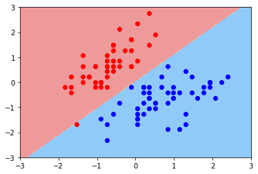
plot_decision_boundary(svc, [-3, 3, -3, 3])
plt.scatter(X_standard[y==0,0], X_standard[y==0,1], color='red')
plt.scatter(X_standard[y==1,0], X_standard[y==1,1], color='blue')
plt.show()
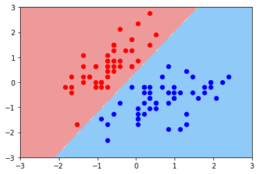
svc2 = LinearSVC(C=0.01)
svc2.fit(X_standard, y)
plot_decision_boundary(svc2, [-3, 3, -3, 3])
plt.scatter(X_standard[y==0,0], X_standard[y==0,1], color='red')
plt.scatter(X_standard[y==1,0], X_standard[y==1,1], color='blue')
plt.show()
svc.coef_
array([[ 4.03240401, -2.49296415]])
svc.intercept_
array([0.95367961])
def plot_svc_decision_boundary(model, axis):
    x0, x1 = np.meshgrid(
        np.linspace(axis[0], axis[1], int((axis[1] - axis[0]) * 100 )).reshape(-1, 1),
        np.linspace(axis[2], axis[3], int((axis[3] - axis[2]) * 100 )).reshape(-1, 1)
    )
    X_new = np.c_[x0.ravel(), x1.ravel()]

    y_predict = model.predict(X_new)
    zz = y_predict.reshape(x0.shape)

    custom_camp = ListedColormap(['#EF9A9A', '#FFF59F', '#90CAF9'])
    plt.contourf(x0, x1, zz, cmap=custom_camp)

    w = model.coef_[0]
    b = model.intercept_[0]

    # w0 * x0 + w1 * x1 + b = 0
    # => x1 = -w0/w1 * x0 - b/w1
    plot_x = np.linspace(axis[0], axis[1], 200)
    up_y = -w[0]/w[1] * plot_x -b/w[1] + 1/w[1]
    down_y = -w[0]/w[1] * plot_x -b/w[1] - 1/w[1]

    up_index = (up_y >= axis[2]) & (up_y <= axis[3])
    down_index = (down_y >= axis[2]) & (down_y <= axis[3])

    plt.plot(plot_x[up_index], up_y[up_index], color='black')
    plt.plot(plot_x[down_index], down_y[down_index], color='black')
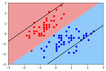
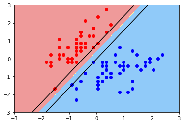
# hard margin
plot_svc_decision_boundary(svc, [-3, 3, -3, 3])
plt.scatter(X_standard[y==0,0], X_standard[y==0,1], color='red')
plt.scatter(X_standard[y==1,0], X_standard[y==1,1], color='blue')
plt.show()
# soft margin
plot_svc_decision_boundary(svc2, [-3, 3, -3, 3])
plt.scatter(X_standard[y==0,0], X_standard[y==0,1], color='red')
plt.scatter(X_standard[y==1,0], X_standard[y==1,1], color='blue')
plt.show()