Stochastic Gradient Descent
April 8, 2019
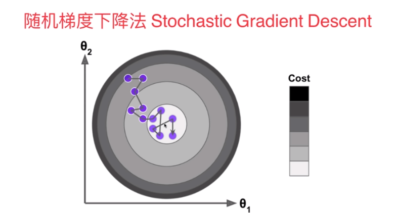
随机梯度下降法
批量梯度下降法(Batch Gradient Descent)
对样本中的所有数据进行计算
样本量很大时很耗时
随机梯度下降法(Stochastic Gradient Descent)
- 抽出一部分样本进行,此时得到的并不是损失函数的梯度,但也代表了一个方向
- 学习率η应该递减
这是一种模拟退火的思想,其中a和b是随机梯度下降法的超参数
- 过程
使用梯度下降法和随机梯度下降法对比
梯度下降
import numpy as np
import matplotlib.pyplot as plt
m = 100000

x = np.random.normal(size=m)
X = x.reshape(-1,1)
y = 4. * x + 3. + np.random.normal(0, 3, size=m)
def J(theta, x_b, y):
    try:
        return np.sum((y - x_b.dot(theta)) ** 2) / len(y)
    except:
        return float('inf')

def dJ(theta, x_b, y):
    return x_b.T.dot(x_b.dot(theta) - y) * 2. / len(y)

def gradient_descent(x_b, y, initial_theta, eta, n_iters=10000, epsilon=1e-8):
    theta = initial_theta
    i_iter = 0
    while i_iter < n_iters:
        gradient = dJ(theta, x_b, y)
        last_theta = theta
        theta = theta - eta * gradient
        i_iter = i_iter + 1
        if(abs(J(theta, x_b, y) - J(last_theta, x_b, y)) < epsilon):
            break
    return theta
%%time
X_b = np.hstack([np.ones((len(x),1)), X])
initial_theta = np.zeros(X_b.shape[1])
eta = 0.01
theta = gradient_descent(X_b, y, initial_theta, eta)
Wall time: 678 ms
theta
array([2.99357905, 4.00121984])
随机梯度下降
def dJ_sgd(theta, x_b_i, y_i):
    return x_b_i.T.dot(x_b_i.dot(theta) - y_i) * 2.
def sgd(x_b, y, initial_theta, n_iters=10000):
    t0 = 5
    t1 = 50
    def learn_rate(t):
        return t0 / (t + t1)
    theta = initial_theta

    for cur_iters in range(n_iters):
        rand_i = np.random.randint(len(x_b))
        gradient = dJ_sgd(theta, x_b[rand_i], y[rand_i])
        theta = theta - learn_rate(cur_iters) * gradient

    return theta
%%time
X_b = np.hstack([np.ones((len(x),1)), X])
initial_theta = np.zeros(X_b.shape[1])
theta = sgd(X_b, y, initial_theta, n_iters=len(X_b) // 3)
Wall time: 229 ms
theta
array([3.05087812, 3.96798923])
使用我们自己封装SGD
%run ../LinearRegression/LinearRegression.py
%run ../util/model_selection.py
X_train, X_test, y_train, y_test = train_test_split(X, y, seed=666)
lr1 = LinearRegression()
lr1.fit_sgd(X_train, y_train, n_iters=2)
LinearRegression()
lr1.coef_
array([3.99577204])
lr1.interception_
2.990127765808477
lr1.score(X_test, y_test)
0.6416976315427425
使用真实数据
from sklearn import datasets
boston = datasets.load_boston()
X = boston.data
y = boston.target
X = X[y < 50.0]
y = y[y < 50.0]
X_train, X_test, y_train, y_test = train_test_split(X, y, seed=666)
from sklearn.preprocessing import StandardScaler
std = StandardScaler()
std.fit(X_train)
X_train_std = std.transform(X_train)
X_test_std = std.transform(X_test)
lin_reg = LinearRegression()
%time lin_reg.fit_sgd(X_train_std, y_train, n_iters=2)
lin_reg.score(X_test_std, y_test)
Wall time: 12 ms
0.7923329555425149
%time lin_reg.fit_sgd(X_train_std, y_train, n_iters=50)
lin_reg.score(X_test_std, y_test)
Wall time: 124 ms
0.8132440489440969
%time lin_reg.fit_sgd(X_train_std, y_train, n_iters=100)
lin_reg.score(X_test_std, y_test)
Wall time: 166 ms
0.8131685005929717
scikit-learn 中的 SGD
from sklearn.linear_model import SGDRegressor
sgd_reg = SGDRegressor(max_iter=5)
%time sgd_reg.fit(X_train_std, y_train)
sgd_reg.score(X_test_std, y_test)
Wall time: 1e+03 µs
0.8047845970157302
sgd_reg = SGDRegressor(max_iter=100)
%time sgd_reg.fit(X_train_std, y_train)
sgd_reg.score(X_test_std, y_test)
Wall time: 16 ms
0.8132804060803719