Use Gradient Descent In Linear Regression
April 6, 2019
在线性回归模型中使用梯度下降法
import numpy as np
import matplotlib.pyplot as plt
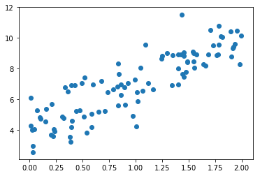
np.random.seed(666)
x = 2* np.random.random(size=100)
y = x * 3. + 4. + np.random.normal(size = 100)
X = x.reshape(-1, 1)
X.shape
(100, 1)
y.shape
(100,)
plt.scatter(x, y)
plt.show()
使用梯度下降法训练
目标:使 \(\frac{1}{m}\sum_{i=1}^m (y^{(i)} - \hat{y}^{(i)})^2\) 尽可能小
\[J(\theta) = MSE(y, \hat{y})\] \[\nabla J(\theta) = \frac{2}{m} \cdot \begin{pmatrix} \sum_{i=1}^m (X_b^{(i)}\theta - y^{(i)}) \\\\ \sum_{i=1}^m (X_b^{(i)}\theta - y^{(i)}) \cdot X^{(i)}_1 \\\\ \sum_{i=1}^m (X_b^{(i)}\theta - y^{(i)}) \cdot X^{(i)}_2 \\\\ \ldots \\\\ \sum_{i=1}^m (X_b^{(i)}\theta - y^{(i)}) \cdot X^{(i)}_n \end{pmatrix}\]def J(theta, x_b, y):
try:
return np.sum((y - x_b.dot(theta)) ** 2) / len(x_b)
except:
return float('inf')
def dJ(theta, x_b, y):
    res = np.empty(len(theta))
    res[0] = np.sum(x_b.dot(theta) - y)
    for i in range(1, len(theta)):
        res[i] = np.sum((x_b.dot(theta) - y).dot(x_b[:,i]))
    return res * 2 / len(x_b)
def gradient_descent(x_b, y, initial_theta, eta, n_iters=10000, epsilon=1e-8):
    theta = initial_theta

    i_iter = 0
    while i_iter < n_iters:
        gradient = dJ(theta, x_b, y)
        last_theta = theta
        theta = theta - eta * gradient
        i_iter = i_iter + 1
        if(abs(J(theta, x_b, y) - J(last_theta, x_b, y)) < epsilon):
            break

    return theta
x_b = np.hstack([np.ones((len(x), 1)), X])
initial_theta = np.zeros(x_b.shape[1])
eta = 0.01

theta = gradient_descent(x_b, y, initial_theta, eta)
theta
array([4.02145786, 3.00706277])
%run ../LinearRegression/LinearRegression.py
lr = LinearRegression()
lr.fit_gd(X, y)
LinearRegression()
lr.interception_
4.021457858204859
lr.coef_
array([3.00706277])