scikit-learn 中的 PCA

import numpy as np
import matplotlib.pyplot as plt
from sklearn import datasets

digits = datasets.load_digits()
X = digits.data
y = digits.target

from sklearn.model_selection import train_test_split
X_train, X_test, y_train, y_test = train_test_split(X, y, random_state=666)

X_train.shape

(1347, 64)

不使用PCA降维，使用knn进行识别，训练时间和精度

%%time
from sklearn.neighbors import KNeighborsClassifier

knn_clf = KNeighborsClassifier()
knn_clf.fit(X_train, y_train)

Wall time: 11 ms

knn_clf.score(X_test, y_test)

0.9866666666666667

使用PCA降维，使用knn进行识别，训练时间和精度

from sklearn.decomposition import PCA

pca = PCA(n_components=2)
pca.fit(X_train)
X_train_reduction = pca.transform(X_train)
X_test_reduction = pca.transform(X_test)

%%time
knn_clf = KNeighborsClassifier()
knn_clf.fit(X_train_reduction, y_train)

Wall time: 1 ms

knn_clf.score(X_test_reduction, y_test)

0.6066666666666667

pca.explained_variance_ratio_

array([0.14566817, 0.13735469])

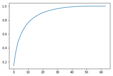
如何确定n_components的值

上述例子可以看到，降维到二维时间大大减少，但是识别精度下降，这不是我们想看到的。

我们可以求出所有主成分，然后根据前n个主成分能够解释的比例来确定

pca = PCA(n_components=X_train.shape[1])
pca.fit(X_train)
pca.explained_variance_ratio_

array([1.45668166e-01, 1.37354688e-01, 1.17777287e-01, 8.49968861e-02, 5.86018996e-02, 5.11542945e-02, 4.26605279e-02, 3.60119663e-02, 3.41105814e-02, 3.05407804e-02, 2.42337671e-02, 2.28700570e-02, 1.80304649e-02, 1.79346003e-02, 1.45798298e-02, 1.42044841e-02, 1.29961033e-02, 1.26617002e-02, 1.01728635e-02, 9.09314698e-03, 8.85220461e-03, 7.73828332e-03, 7.60516219e-03, 7.11864860e-03, 6.85977267e-03, 5.76411920e-03, 5.71688020e-03, 5.08255707e-03, 4.89020776e-03, 4.34888085e-03, 3.72917505e-03, 3.57755036e-03, 3.26989470e-03, 3.14917937e-03, 3.09269839e-03, 2.87619649e-03, 2.50362666e-03, 2.25417403e-03, 2.20030857e-03, 1.98028746e-03, 1.88195578e-03, 1.52769283e-03, 1.42823692e-03, 1.38003340e-03, 1.17572392e-03, 1.07377463e-03, 9.55152460e-04, 9.00017642e-04, 5.79162563e-04, 3.82793717e-04, 2.38328586e-04, 8.40132221e-05, 5.60545588e-05, 5.48538930e-05, 1.08077650e-05, 4.01354717e-06, 1.23186515e-06, 1.05783059e-06, 6.06659094e-07, 5.86686040e-07, 1.71368535e-33, 7.44075955e-34, 7.44075955e-34, 7.15189459e-34])

plt.plot([i for i in range(X_train.shape[1])], [np.sum(pca.explained_variance_ratio_[:i+1]) for i in range(X_train.shape[1])])
plt.show()

sklearn 中 PCA支持直接设置解释率

pca = PCA(0.95)
pca.fit(X_train)

PCA(copy=True, iterated_power=’auto’, n_components=0.95, random_state=None, svd_solver=’auto’, tol=0.0, whiten=False)

pca.n_components_

28

X_train_reduction = pca.transform(X_train)
X_test_reduction = pca.transform(X_test)

%%time
knn_clf = KNeighborsClassifier()
knn_clf.fit(X_train_reduction, y_train)

Wall time: 2 ms

knn_clf.score(X_test_reduction, y_test)

0.98

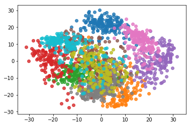
降到二维的意义–可视化

会看到在数据是二维的时候，某些数字所在的样本空间和其他区分很开

pca = PCA(n_components=2)
pca.fit(X)
X_reduction = pca.transform(X)

X_reduction.shape

(1797, 2)

for i in range(10):
    plt.scatter(X_reduction[y==i,0], X_reduction[y==i,1], alpha=0.8)
plt.show()